Reducing IoT data bills using Compression and Batching- Part 3

Welcome to Part 3 of our multipart guide. In this instalment, we continue our exploration of techniques to optimize the transmission of data from IoT devices to the cloud. Building upon the fundamentals of serialization and compression discussed in Part 1 and the performance analysis of serialization covered in Part 2, we will now focus on data compression and batching.
In today's data-driven world, IoT devices are ubiquitous, generating unprecedented volumes of data. From your refrigerator to your smartwatch, a wide array of devices continuously send vital data to the cloud. It's crucial to understand how to make the most efficient use of network resources, whether it's over WiFi or cellular connections. By leveraging the principles we've explored so far, you can substantially reduce your network bills – potentially saving up to 75% of your costs.
Recap of Part 2
In Part 2, we conducted a comprehensive performance analysis of various serialisation techniques and data formats. This analysis provided invaluable insights into the efficiency of data serialization, on different data types, such as IMU data, GPS data, motor data, and battery management system (BMS) data. We closely examined data size and latency during transmission after the serialization process. Experiments performed in Part 2 conclude that Schema-based serialization, notably Capnproto, excels with smaller data size and superior serialization speed in all tests.
What to Expect from this guide: In this guide, we'll conduct a performance analysis of compression and batching techniques. Our focus will be on size and time-based assessments, for different kinds of data types like GPS data, BMS data, IMU data and motor data.
The different levers of reducing data size
There are 2 levels when it comes to reducing the size of data to be transferred over the network, they are:
- Serialisation
- Compression
Earlier, in Part 1 of this multi-part series, We have made a comprehensive guide on compression and serialization concepts, Check out Part 1 to deep dive into concepts of Serialization and compression.
In this article, we will look at how serialization affects the size of data and how all of it depends on the nature of the data being transmitted. In Part 3 of this multipart guide, we will look at the compression and batching process and How it affects the size of the data and the latency associated with it.
Introducing the Compression and Batching Experiments.
To help us better understand the relationship between the different types of data and the different compression and serialization formats that can be used on it, we set up an experiment called Zerde. To simulate the different types of data, we wrote a simulator that generates random IMU, BMS and perStatus values while also emulating GPS data from a set of real-world coordinates, hard-coded into a CSV file and then plotting this data on 3D bar charts.
The simulator ensures that it sends data points at the expected frequency, according to the type of data, i.e. GPS data is produced slower than BMS/IMU data. Data is sent onto a stream where it is batched and forwarded to the serialisation modules as a “data buffer”, we will now discuss the rest of the steps in the following sections.
Further, To understand the effect of batching on the size of data and time taken for compression and decompression, We have bundled our data in batches of 10, 100 and 1000. We will carry out compression+serialization and decompression+deserialization experiments in batches of 10,100 and 1000.
Compression Experiment
Various sensors generate data at distinct frequencies. Like raw motion data or IMU data, it could be more frequent than data from GPS. It is generally a good practice to batch the data before transmission to the cloud. This batching process optimizes the efficiency of data transfer, ensuring a streamlined and resource-efficient flow of information.
For this experiment, we have considered a batch size of 100. Each element of the batch contains about 52 data points for the following data type:
| Sensor Profile | Type of data | Size of Data |
|---|---|---|
| GPS | Latitude and longitude data from moving vehicle | 820 bytes to 840 bytes |
| IMU | Accelerometer and Gyroscope data | 260 bytes to 280 bytes |
| BMS | Voltage Current and temperature data | 1300 bytes to 1400 bytes |
| Motor | RPM and vibration velocity data | 208 bytes to 210 bytes |
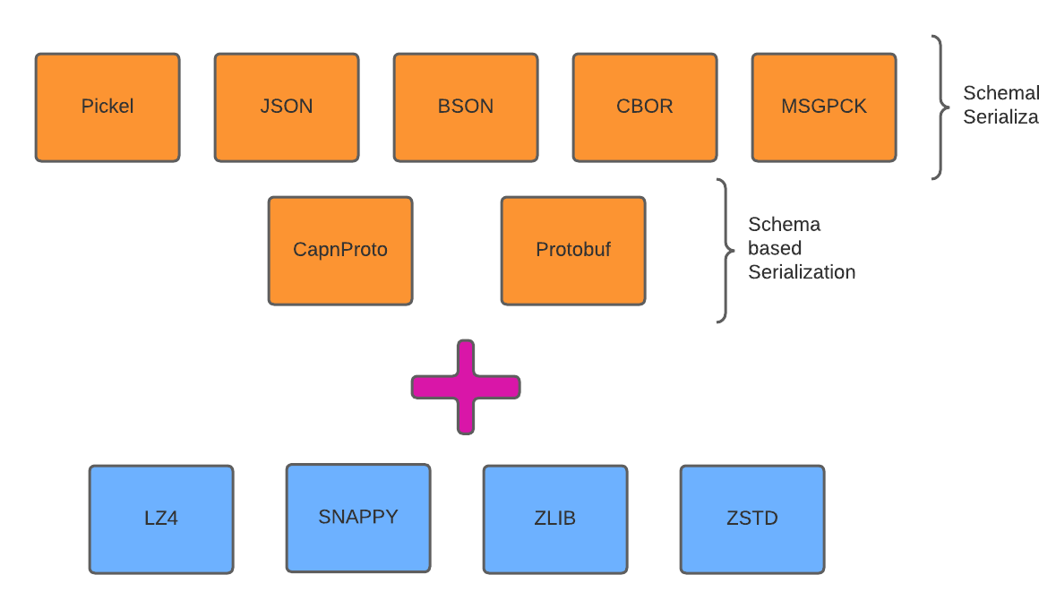
In this experiment, we are employing a combination of serialization and compression techniques on the data sample to choose the best techniques among all. We will be combining different schema-based serialization and schema-less serialization techniques with different compression algorithms. The figure below shows this combination
Next, we will be showing you the experiment results for the following in batches of 10, 100 and 1000
- Size of payloads after serialization and compression
- Time taken for serialization and compression
- Time taken for de-serialization and de-compression
Compression + Serialization performance analysis: Size of Data
After running the experiments. The graphs shown below interpret the following insights.
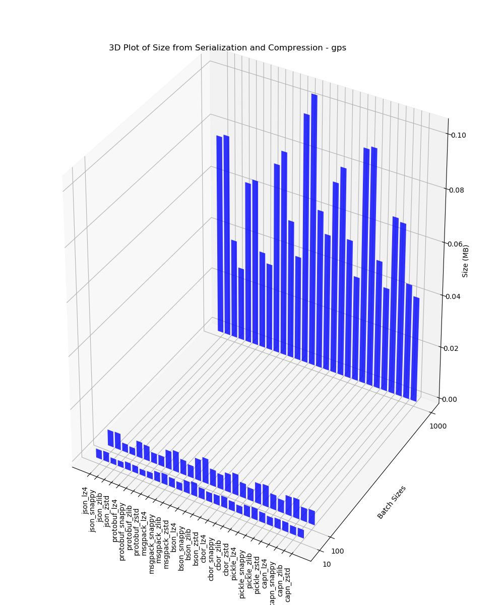
- Amongst different compression algorithms, zstd and zlib emerge as the frontrunners, boasting a marginal advantage. Notably, zstd produces a smaller size output out of all.
- Looking at serialization techniques when used with compression algorithms, in some cases the distinction between schema-based and schema-less approaches has minimal variations in output size. Interestingly, certain schema-less techniques, such as cbor, exhibit superior performance over their schema-based counterparts.
- Visualizing our findings in the graph below shows that combinations involving cbor and zstd yield notably smaller outputs when compared with alternative configurations. Similarly, the fusion of Capnproto and zstd also proves to be a good contender. This experiment shows that lz4 and snappy compression algorithms produce larger outputs as compared to others.
GPS
This 3D plot contains the size of data analysis after serialization and compression for batches of 10, 100 and 1000 performed on GPS data
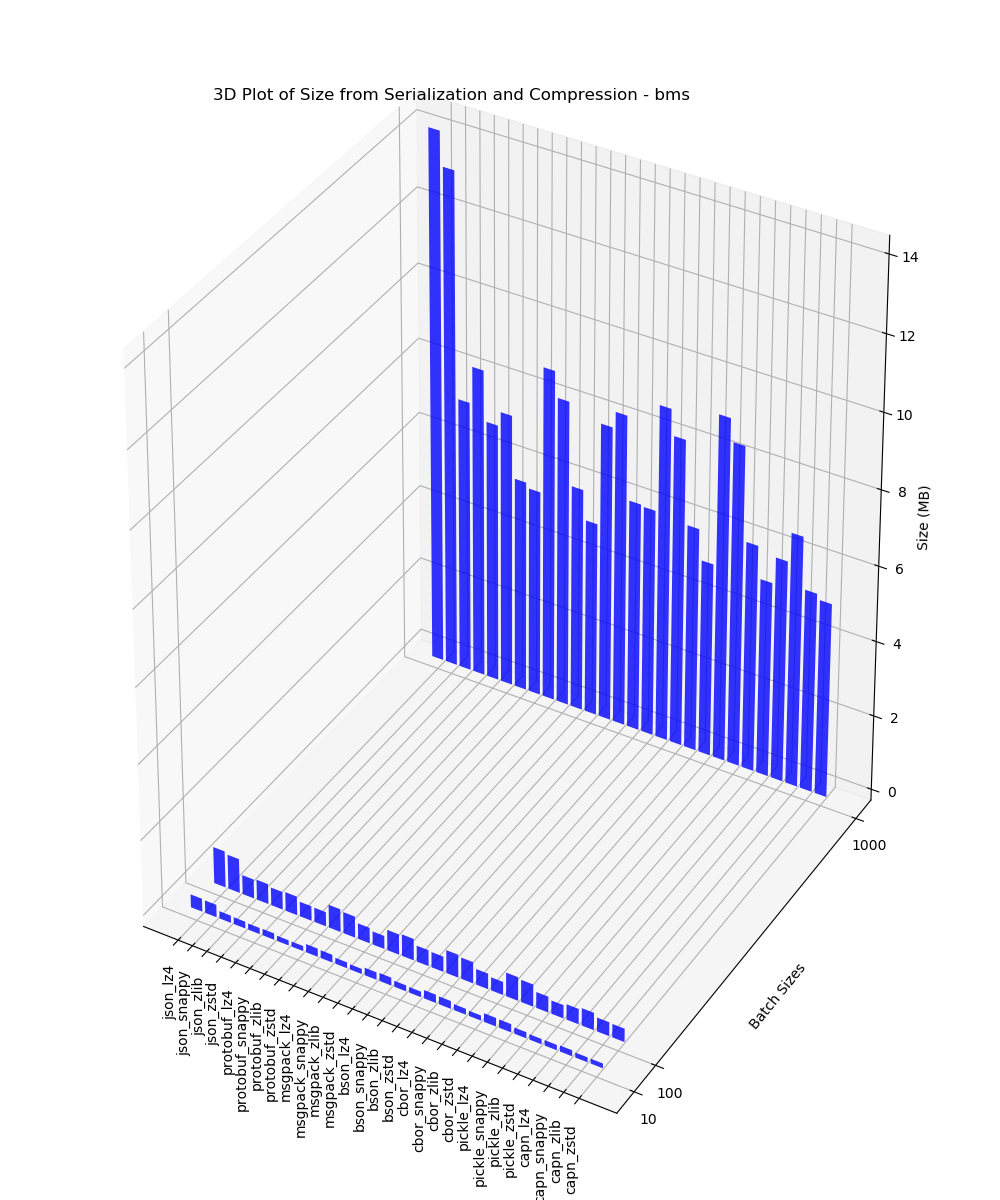
BMS
This 3D plot contains the size of data analysis after serialization and compression for batches of 10, 100 and 1000 performed on BMS data
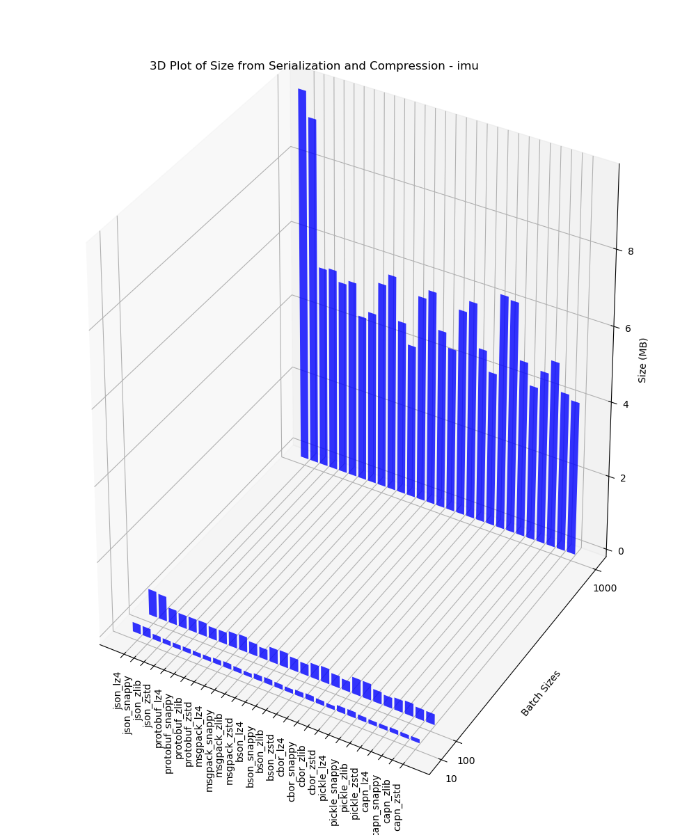
IMU
This 3D plot contains the size of data analysis after serialization and compression for batches of 10, 100 and 1000 performed on IMU data
Compression + Serialization performance analysis: Time
After running the experiments. The graphs shown below interpret the following insights.
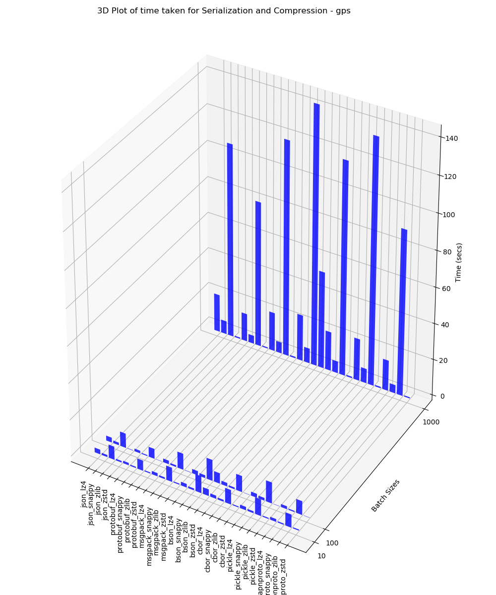
- Amongst the array of compression algorithms available, zstd stands out as the clear champion, taking less time to compress as compared to its counterparts.
- Other than zstd, snappy also takes comparatively less time for compression.
- The graph below displays the superiority of combinations featuring capnproto and zstd, consistently yielding smaller outputs when compared to other pairings. Similarly, the partnership of pickel and zstd also demonstrates enhanced performance.
- However, it's worth noting that our experiments reveal that the zlib compression algorithm consistently takes a longer time to compress in comparison to its counterparts, making it a less favourable choice in this context.
GPS
This 3D plot contains the time taken for serialization and compression analysis for batches of 10, 100 and 1000 performed on GPS data
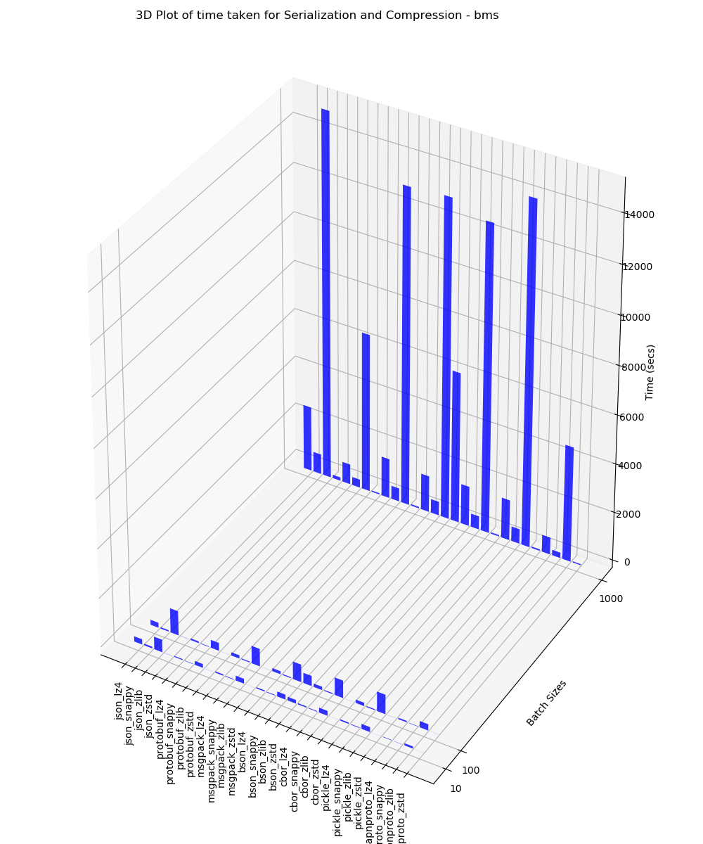
BMS
This 3D plot contains the time taken for serialization and compression analysis for batches of 10, 100 and 1000 performed on BMS data
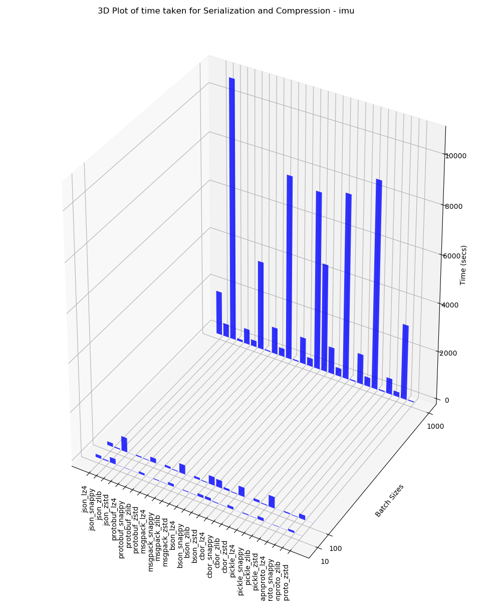
IMU
This 3D plot contains the time taken for serialization and compression analysis for batches of 10, 100 and 1000 performed on IMU data
De-Compression + De-Serialization performance analysis: Time
After running the experiments. The graphs shown below interpret the following insights.
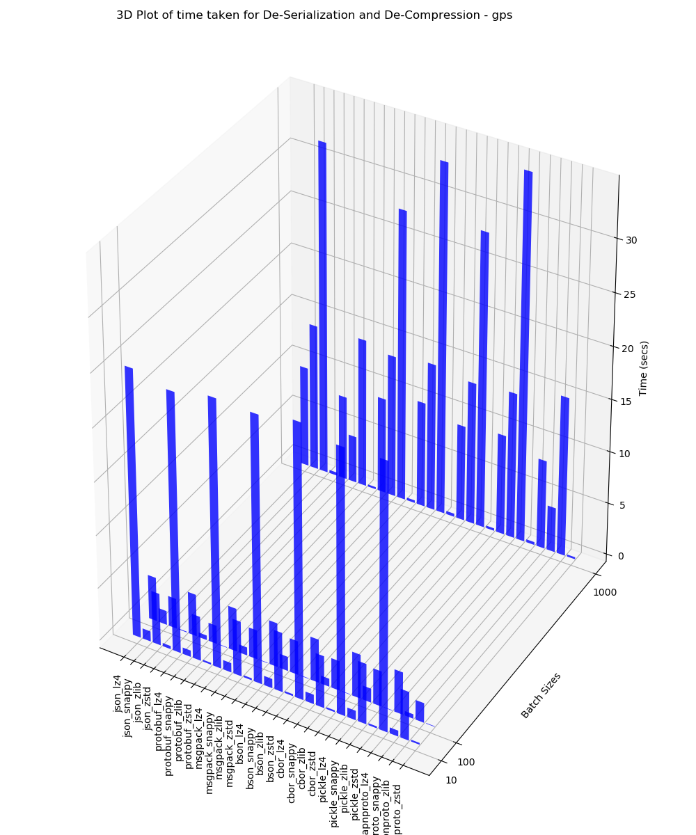
- When it comes to decompression, one clear standout is the zstd algorithm. It consistently outpaces its competitors by completing the process in less time.
- Apart from zstd, another speedy contender is snappy, which also excels in reducing compression time.
- The graph below vividly illustrates that combinations involving capnproto and zstd consistently outperform other pairings, boasting faster execution times. Similarly, the duo of pickel and zstd showcases impressive performance.
- It's worth noting that our experiments consistently show that the zlib compression algorithm tends to take more time for decompression compared to its counterparts. This places zlib as a less favourable choice in the context of our experiments.
GPS
This 3D plot contains the time taken for de-serialization and de-compression analysis for batches of 10, 100 and 1000 performed on GPS data.
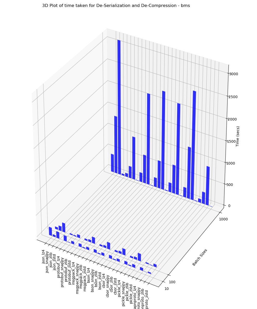
BMS
This 3D plot contains the time taken for de-serialization and de-compression analysis for batches of 10, 100 and 1000 performed on BMS data
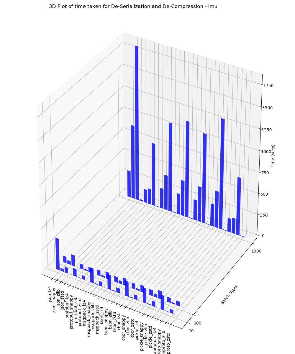
IMU
This 3D plot contains the time taken for de-serialization and de-compression analysis for batches of 10, 100 and 1000 performed on IMU data
Results Summary
Here is the result summary for the experiments performed above.
Compression and Serialization
Our experiments have yielded compelling insights. Firstly, zstd consistently outperforms other methods across all three tests. Secondly, the combination of cbor and zstd impressively reduces output sizes compared to alternative configurations. When it comes to compression and decompression speed, the capnproto and zstd pairing emerges as the fastest, and similarly, the duo of pickel and zstd showcases noteworthy performance in decompression and deserialization. These findings underscore the efficacy of zstd and provide essential guidance for optimizing data compression and manipulation techniques to enhance efficiency and minimize data footprint.
Batching
Our experiments revealed the transformative impact of data batching on compression and serialization. We compared batches of 10 and 100, discovering that larger batches yielded remarkably smaller data sizes, though with a marginal increase in compression and serialization time. We also found that high-frequency data such as GPS data performs better. Thus, larger batch sizes are to be preferred for higher-frequency data.
Practical considerations
As mentioned earlier, we have to keep in mind the practical effects of our decisions when choosing the right serialisation and compression formats, as well as the batch size. These are a few points to keep in mind:
- Batch size vs frequency: the higher the frequency, the larger the batch size.
- Availability of libraries: We found that a few libraries are unavailable for languages or practically impossible to integrate into our use case, it is important to keep this in mind while choosing the right format for serialisation or compression in your application.
- Constraints on microcontrollers: constraints such as smaller memory or lower processing power will significantly affect its ability to serialise or compress data efficiently.
Conclusion
In this post, we learned that zstd stands out among all other compression algorithms. CapnProto and zstd yield notably smaller outputs when compared with alternative configurations. Also, during batching, we found that larger batch sizes are to be preferred for higher-frequency data. The exact solution depends on your use case.
Bytebeam offers a comprehensive suite of features and tools to enhance your IoT and data management experience. Check out our data Visualization guide for creating interactive dashboards, OTA guide for remote updates and the Handling Action Guide for remote operations.
I hope you find this guide useful. As we continue to come up with more interesting tutorials and maker content, we invite you to explore Bytebeam further and see how our platform can empower your projects.
Stay tuned!


