Reducing IoT data bills using Serialization - Part 2

IoT devices are everywhere and they are generating more data than has ever been generated in the history of humankind. With everything from a fridge to a smartwatch sending vital data to the cloud, it is important to ensure there is a proper understanding of how to better utilise the network as a resource. The network in this case can refer to either Wi-Fi or Cellular.
Earlier, In Part 1 of this multipart guide, we got an overview of data serialization and compression. By employing these techniques, you can better utilize the network’s bandwidth and can save up to 75% of your bills. In this guide, we will see the effect of various data serialization formats on data transmission sizes.
What to Expect from this guide
In this guide, we'll conduct a performance analysis of data serialization formats. Our focus will be on size and time-based assessments, for different kinds of data types like GPS data, BMS data, IMU data, and motor data.
So let's get started.
Nature of data
Not all data is made equally, devices collect data from all kinds of sensors, some of these are mentioned below:
- High-frequency fast-moving data: an IMU sensor can produce several hundred data points per second.
- Low-frequency fast-moving data: a GPS module produces around one data point per second.
- Very slow-moving data: component statuses or action notifications are typically transmitted at an even lower frequency, of say, a data point once every few seconds or even once every few minutes.
What's the Story So Far? Part 1 Recap
In the first instalment of our exploration into optimizing IoT efficiency, Part 1 provided a comprehensive overview of Serialization and Compression concepts. You can revisit the details in Part 1. The blog covered an array of Serialization and Compression formats, demystifying the core concepts essential for reducing data bills in the IoT landscape. Part 1 laid the groundwork for a solid grasp on these fundamentals Serialisation and Compression. If you haven't dived into the details yet, catch up on the basics and kickstart your journey to mastering IoT optimization in Part 1.
Introducing the Zerde Simulator
To help us better understand the relationship between the different types of data and the different serialisation formats that can be used on it, we set up an experiment called Zerde. To simulate the different types of data, we wrote a simulator that generates random IMU, BMS, and Motor values while also emulating GPS data from a set of real-world coordinates, hard-coded into a CSV file, and then plotting this data on a bar chart.
The simulator ensures that it sends data points at the expected frequency, according to the type of data, i.e. GPS data is produced slower than BMS/IMU data. Data is sent onto a stream where it is batched and forwarded to the serialisation modules as a “data buffer”, we will now discuss the rest of the steps in the following sections.
Experiment Setup
Various sensors generate data at distinct frequencies. Like raw motion data or IMU data, it could be more frequent than data from GPS. It is generally a good practice to batch the data before transmission to the cloud. This batching process optimizes the efficiency of data transfer, ensuring a streamlined and resource-efficient flow of information.
For this experiment, we have considered a batch size of 100. Each element of the batch contains about 52 data points for the following data type:
| Sensor Profile | Type of data | Size of Data |
|---|---|---|
| GPS | Latitude and longitude data from moving vehicle | 820 bytes to 840 bytes |
| IMU | Accelerometer and Gyroscope data | 260 bytes to 280 bytes |
| BMS | Voltage Current and temperature data | 1300 bytes to 1400 bytes |
| Motor | RPM and vibration velocity data | 208 bytes to 210 bytes |
Next, we will be showing you the experiment results for the following
- Size of payloads after serialisation.
- Time taken for serialisation.
- Time taken for de-serialisation
Size of Serialized Data
The amount of data after serialization directly impacts your data bills. So, making the data smaller by techniques like batching can help you save costs. But, it might take a bit more time to process. Finding the sweet spot means optimizing the data size without losing crucial information, ensuring a cost-effective approach to transmitting data.
Time taken for serialization
The time it takes to serialize data is a critical factor. While we aim for smaller data for cost savings. It comes with a trade-off – it might take a bit longer to serialize. Striking the right balance is key, ensuring that the serialization process is not just efficient but also timely for real-time responsiveness.
Time taken for de-serialization
The time it takes to de-serialize data is a significant consideration for server costs. Streamlining this process is essential because extra time spent on de-serialization can lead to higher server bills. It's about finding the right speed without overloading servers, and managing costs efficiently while maintaining optimal processing speed.
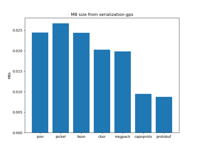
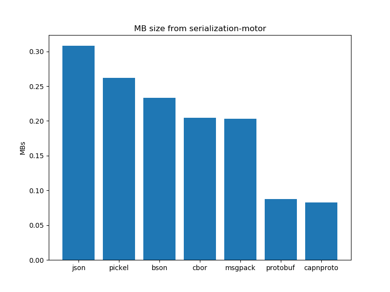
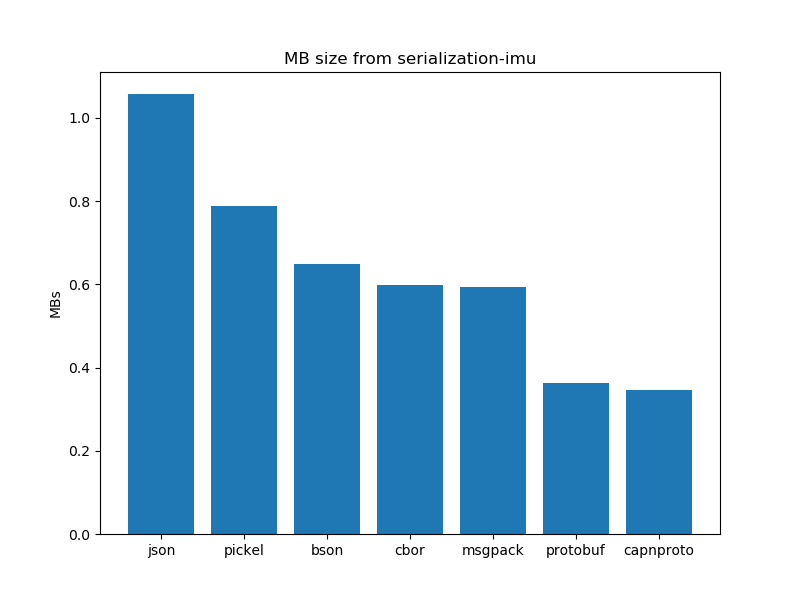
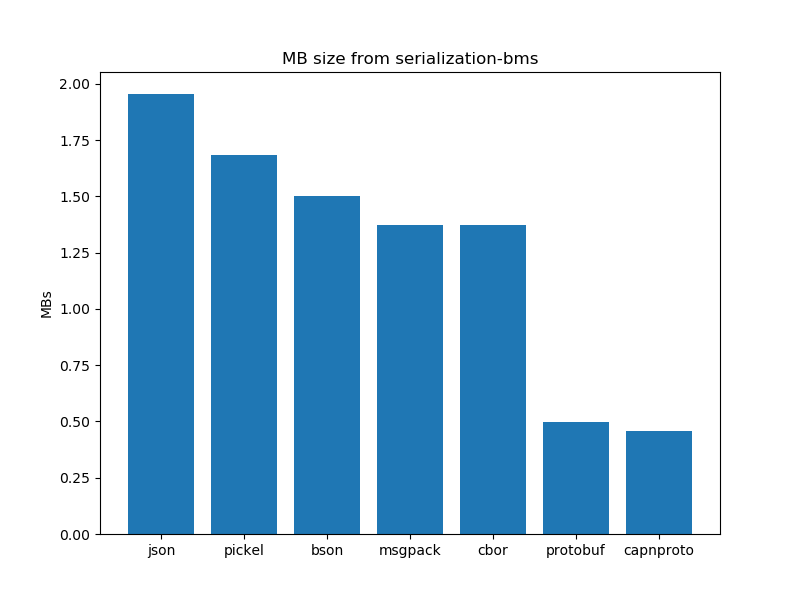
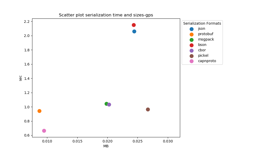
Data Serialization performance analysis: Size of data
After running the experiments. The graphs shown below interpret the following insights.
- In general, certain schema-based serialization formats produce a smaller serialised output than their schemaless alternatives.
- In the case of schema-based serialization formats capnproto shows better results as compared to protobuf.
- In the case of schema-less serialization formats, cbor presents us with better results as compared to bson and other schema-less formats. JSON and pickel produce larger outputs as compared to their other counterparts.
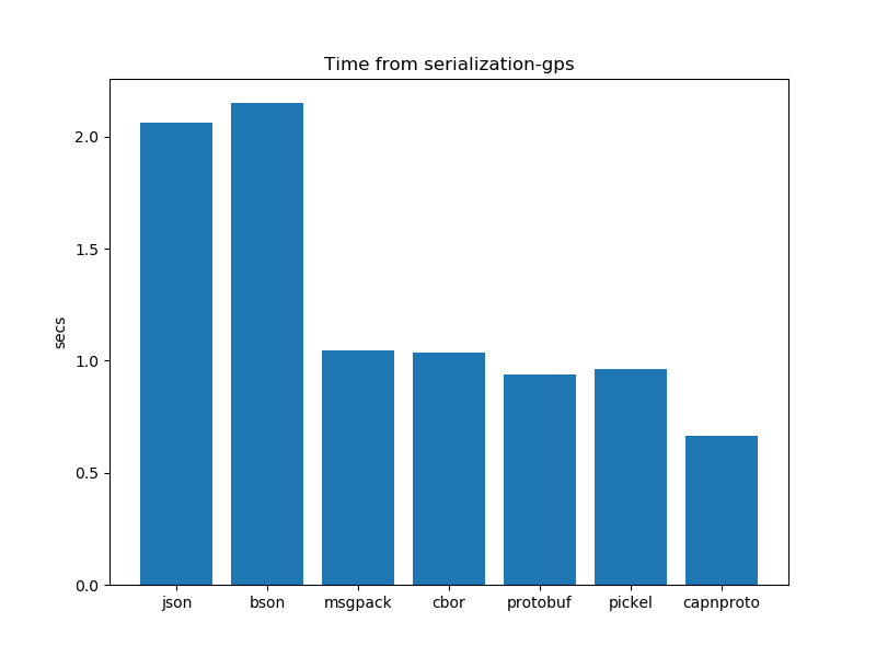
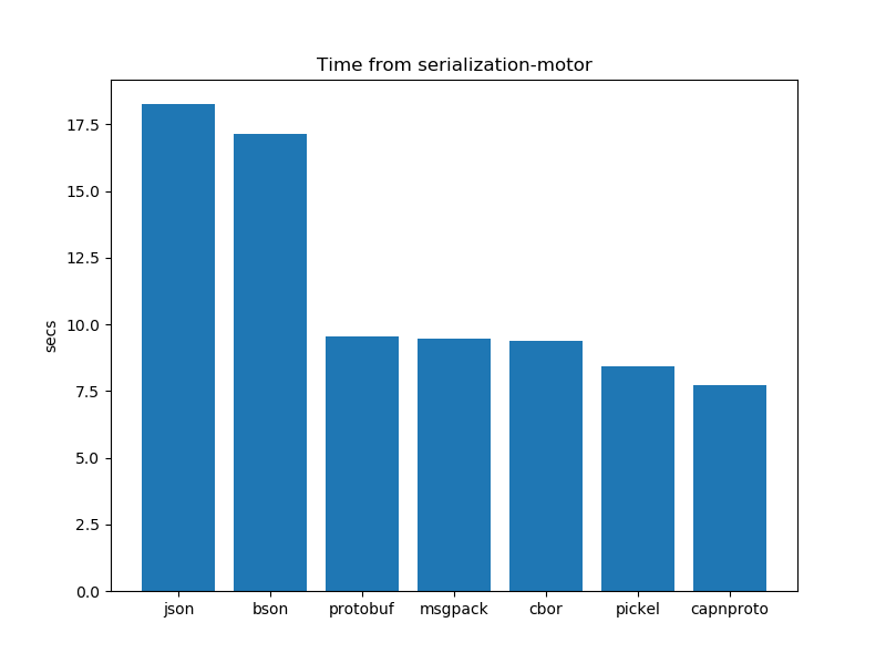
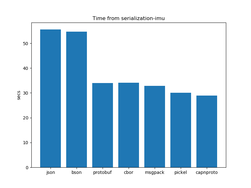
Serialisation performance analysis: Time
After running the experiments. The graphs shown below interpret the following insights.
In general, there is not a clear winner between schema-based serialization and schema-less serialization. Both have mixed results. However, Pickel takes the least amount of time out of all other formats.
- In the case of schema-based serialization formats capnproto takes less time for serialization as compared to protobuf
- In the case of schema-less serialization formats pickel presents us with better results and takes the least time as compared to its other counterparts. bson and JSON take more time for serialization.
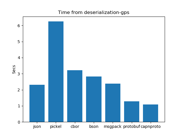
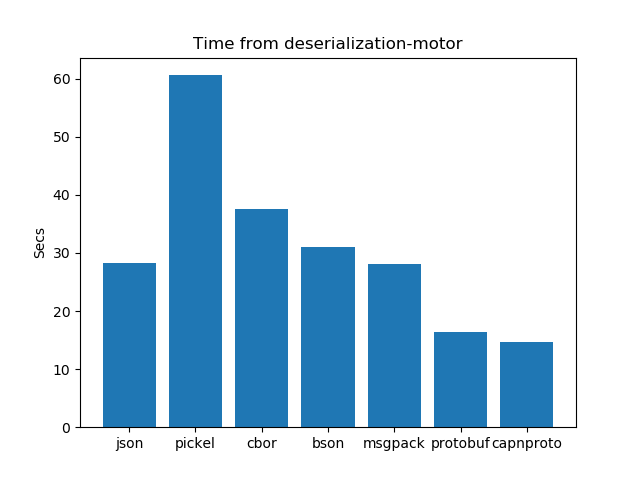
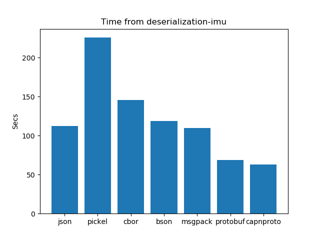
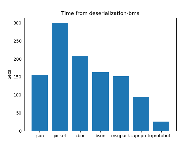
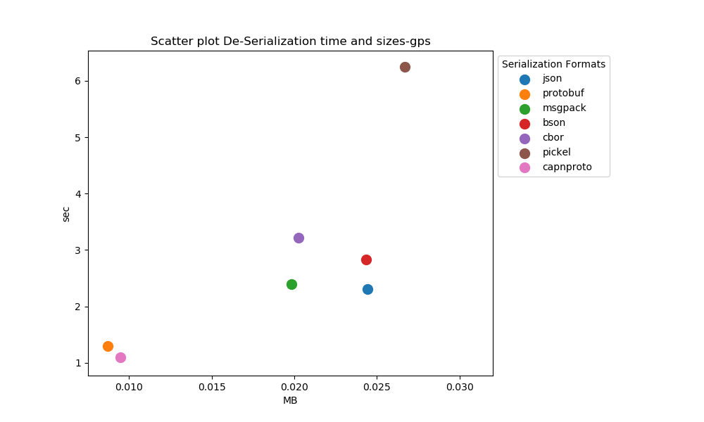
De Serialization performance analysis: Time
After running the experiments. The graphs shown below interpret the following insights.
- In the case of De-serialization schema-based formats have an edge over schema-less formats. Protobuf works better and takes the least time as compared to all other formats.
- In the case of schema-based serialization formats protobuf takes less time for serialization as compared to capnproto.
- In the case of schema-less serialization formats msgpck and cbor present us with better results and take the least time as compared to their other counterparts. Pickel and BSON take more time for de-serialization.
Results Summary
After carefully analyzing the experiments mentioned above, we can make some important observations:
Schema-based serialization methods consistently outperform schema-less techniques in all three tests. Among the various serialization methods, Capnproto stands out by producing the smallest serialised data compared to the others. When it comes to serialization speed, Protobuf and Capnproto take the lead, showing excellent performance. In the deserialization process, Protobuf proves to be the fastest, requiring the least amount of time. In essence, these findings provide valuable insights into the most effective choices for data serialization and deserialization, which are vital aspects of optimizing data handling and efficiency.
Practical considerations
As mentioned earlier, we have to keep in mind the practical effects of our decisions when choosing the right serialisation and compression formats, as well as the batch size. These are a few points to keep in mind:
- Batch size vs frequency: the higher the frequency, the larger the batch size.
- Availability of libraries: We found that a few libraries are unavailable for languages or practically impossible to integrate into our use case, it is important to keep this in mind while choosing the right format for serialisation or compression in your application.
- Constraints on microcontrollers: constraints such as smaller memory or lower processing power will significantly affect its ability to serialise or compress data efficiently.
Conclusion
In this post, we learned that schema-based serialisation formats produce smaller outputs and are generally faster. CapnProto stands out as the best serialisation technique, it produces the smallest serialised data. The exact solution depends on your use case. In part 3 of this multipart guide, We will do the performance analysis of compression techniques. We will also look at the batching process and how it affects the size and time factors.
Bytebeam offers a comprehensive suite of features and tools to enhance your IoT and data management experience. Check out our Data Visualisation guide for creating interactive dashboards, OTA guide for remote updates and the Handling Action Guide for remote operations.
I hope you find this guide useful. As we continue to come up with more interesting tutorials and maker content, we invite you to explore Bytebeam further and see how our platform can empower your projects.
Stay tuned!


